Coagent Networks

Training a neural network without backpropagation

Coagent Network and Global REINFORCE

Most deep learning methods nowadays are based on training a neural network through backpropagation. Despite backpropagation’s effectiveness, it is widely considered biologically implausible. For instance, it is hard to imagine how a biological neuron could send two signals—one forward and one backward—synchronously throughout the entire network. Neuroscience studies suggest that a biological neuron’s learning rule is largely local, meaning that the learning rule mostly depends on pre-synaptic and post-synaptic activation (i.e., the inputs and outputs of a neuron), modulated by some global factors. Is it possible to train an artificial neural network using local learning rules?

The answer is yes. An alternative way of training a network involves treating each neuron as an RL agent, where all RL agents learn from the same reward. Each neuron independently explores and attempts to correlate its action with the global reward. I will refer to this method as Global REINFORCE in this article. This idea was proposed back in the 1973 by Tsetlin and further extended to multi-layer networks by Barto in 1985 .

Let’s examine the details of Global REINFORCE. Consider a simplified RL setting with a single time step (equivalent to contextual bandits), where the state, action, and reward are denoted by \(S\), \(A\), and \(R\).The learning rule in this article can all be generalized to the general RL setting, by replacing the reward with TD errors. For supervised learning, replace the reward with the negative loss. We aim to learn the parameter \(W\) such that when an action is sampled from the policy function \(\pi(s, a \vert W) = \text{Pr}(A=a \vert S=s ; W)\) , the expected reward \(\mathbb{E} [R \vert \pi]\) is maximized.

It can be shown that:

\[\nabla_W \mathbb{E} [R \vert \pi] = \mathbb{E} [R \nabla_{W}\log \text{Pr}(A|S; W) \vert \pi],\]

which leads to the REINFORCE learning rule , with \(\alpha > 0\) denoting the learning rate:

\[W \leftarrow W + \alpha R \nabla_{W}\log \text{Pr}(A|S; W),\]

This learning rule is intuitive. We perform gradient ascent on the probability of selecting the chosen action, scaled by the return. This update causes the parameters to move towards the directions that favor the action with the highest return. In other words, if the reward is positive, we increase the probability of repeating the same action, and vice versa.

Fig 1: Conventional and an alternative view of a policy function parameterized by a multi-layer feedforward neural network.

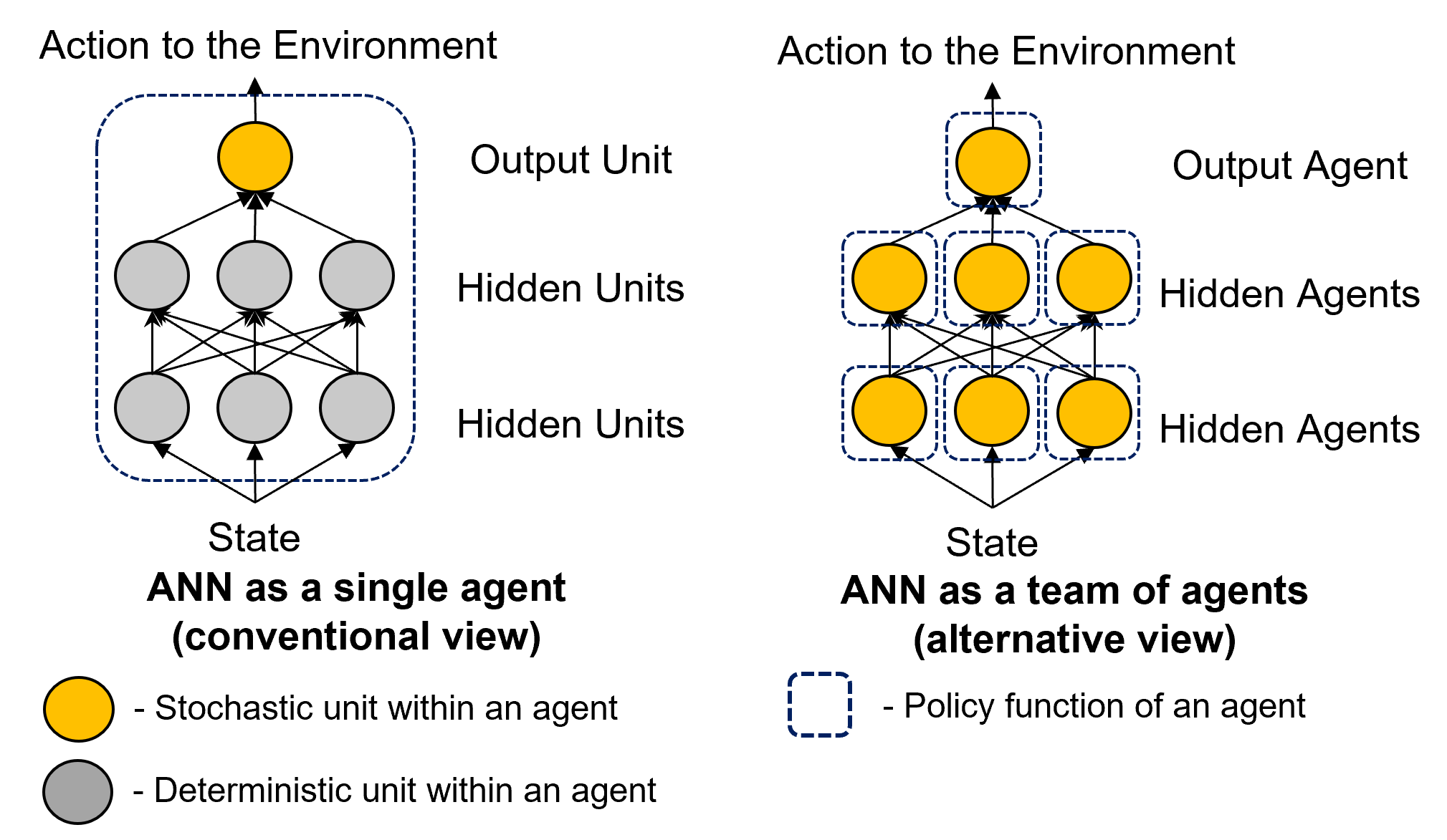
Now, consider a policy function parameterized by a multi-layer feedforward neural network, as shown in Figure 1 (left). Conventionally, the hidden units are deterministic, and only the output unit is stochastic, necessary for the agent to explore. We treat the entire network as a single agent and apply the REINFORCE learning rule. Specifically, the gradient of a hidden unit’s weight on the expected reward can be computed through backpropagation from the top layer. In this article, I refer to this method simply as backpropagation.

Alternatively, consider each hidden unit as stochastic and treat each unit in the network as an agent. For each hidden unit, the layer immediately below can be considered the state, the action selected as the output of the hidden unit, and all other layers as part of the black-box environment, as shown in Figure 1 (right). Such a network of agents is called a coagent network .

Based on this alternative view of the environment for each unit, we can simply apply the REINFORCE learning rule to each unit:

\[W^l \leftarrow W^l + \alpha R \nabla_{W^l}\log \text{Pr}(H^l|H^{l-1}; W^l),\]

where \(W^l\) denotes the weight of layer \(l\), and \(H^l\) denotes the activation values of hidden units in layer \(l\) (we let \(H^0 = S\) and \(H^L = A\), with \(L\) being the number of layers in the network).

We refer to this neural network training method as Global REINFORCE. This approach is sometimes called perturbation learning, as it essentially involves perturbing each neuron’s activity and updating its weight based on an estimated correlation. The Global REINFORCE learning rule is a three-factor rule, depending solely on: (i) the pre-synaptic activation, (ii) the post-synaptic activation, and (iii) the global reward. This bears a strong resemblance to R-STDP (Reward-modulated Spike-Timing-Dependent Plasticity) , discovered in brains in the 2000s. While it is a simple and elegant learning rule, it has a significant drawback: it is extremely slow.

Inefficient Structural Credit Assignment

Consider a scenario where a professor, instead of providing individual assignment grades, only informs students about the average grade of the entire class. Theoretically, it’s possible to correlate your performance with this average grade, but such a correlation would be inherently noisy. If you were the sole student in the class, the correlation might still be easy to estimate. However, as the number of students increases, determining your actual performance becomes increasingly challenging. A similar issue arises with Global REINFORCE, where all units essentially receive the same global reward. This challenge is known as structural credit assignment. In Global REINFORCE, every unit receives the same credit, whereas in backpropagation, each unit receives precise credit based on its influence on the final action. This distinction explains why Global REINFORCE does not scale well with the number of units in a network, as compared to backpropagation:

Fig 2: Performance of Global REINFORCE and Backpropagation on the multiplexer task. Global REINFORCE scales poorly with the size of the network.

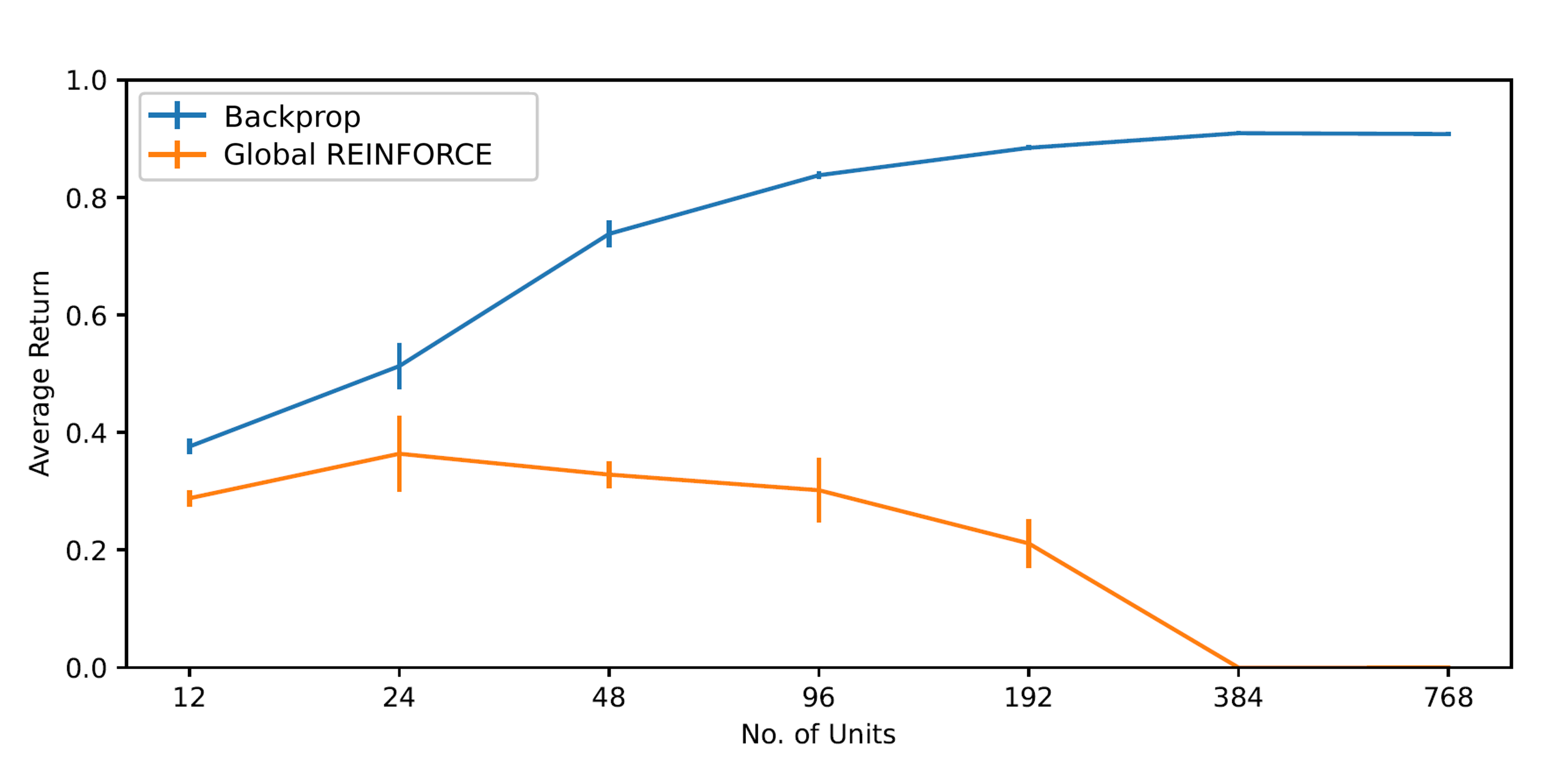
This presents a dilemma: Global REINFORCE is biologically plausible but impractical due to its slow speed, while backpropagation is effective in practice but biologically implausible. Many studies have attempted to revise backpropagation to make it more biologically plausible. However, we approach this from the opposite end—how can we make Global REINFORCE more practical? Specifically, are there ways to improve the learning speed of Global REINFORCE? Our investigation into various methods highlighted two particularly promising approaches: Weight Maximization and MAP Propagation .

Weight Maximization

The concept of Weight Maximization is relatively straightforward. We modify the reward for each hidden unit to reflect the change in the norm of its outgoing weights (i.e., the weights of the layer above). In this method, each hidden unit in the network tries to maximize the norm of its outgoing weights rather than the global returns. The underlying intuition is that the norm of a unit’s output weights approximately represents its utility. For instance, if a unit is effective in guiding action, then the outgoing units will learn to associate a large weight with it. Conversely, if a unit is producing random noise, the outgoing units will assign a negligible weight to it. As each unit aims to maximize the norm of its output weights, it also maximizes its utility within the network.

The learning rule for Weight Maximization in hidden units of layer \(l\) is given by:

\[W^l \leftarrow W^l + \alpha R^l\nabla_{W^l}\log \text{Pr}(H^l|H^{l-1}; W^l),\]

where \(R^l\) represents the change in the norm of the outgoing weight, a vector due to the presence of multiple units in layer \(l\). The \(i^{th}\) entry of \(R^l\) is given by:

\[R^l_{i} = \sum_{j} \| W^{l+1}_{ij} + \Delta W^{l+1}_{ij} \|^{2} - \| W^{l+1}_{ij} \|^{2},\]

with \(\Delta W^{l+1}\) denoting the weight update to layer \(l+1\) and \(W^{l+1}_{ij}\) being the weight connecting unit \(i\) in layer \(l\) to unit \(j\) in layer \(l+1\).

Our paper demonstrates that this learning rule approximates the gradient of reward in expectation. We can interpret this as all units competing to be useful, as measured by the norm of their outgoing weights. This contrasts with the original Global REINFORCE, where every unit receives the same reward. Nevertheless, it is still fundamentally based on Global REINFORCE, as we only replace the global reward with a unit-specific local reward.

Although Weight Maximization is conceptually simple, layer-wise synchronization remains necessary, as updates to all upper layers must be completed before determining the change in the norm of the outgoing weights. To address this, we also propose integrating eligibility traces to eliminate such requirements. Eligibility traces offer a simple yet effective solution for dealing with delayed rewards in general. The paper provides more details on combining eligibility traces with Weight Maximization. Ultimately, the task of maximizing the outgoing weights is a local problem, one that does not necessitate any backward signals from above, as is required in backpropagation.

MAP Propagation

Weight Maximization involves designing a specific reward for each unit, while each unit still explores independently. Another direction is using the same global reward but allowing each unit to explore in a coordinated manner.

Imagine playing a computer game with a controller that has only two buttons (A and B). When you press one of these buttons, there’s a 5% chance the opposite button will be transmitted to the computer instead. Now, suppose you pressed button A, but the computer indicates you pressed button B, and then you receive a large reward. What should you press the next time you encounter the same situation? Intuitively, you should press button B to collect the large reward, because it’s more likely that button B was pressed, despite that you actually pressed button A.

This leads to the following idea: the true action selected by a hidden unit is not important; only the most probable action selected by the hidden unit, conditioned on the final action (the one passed to the environment), matters. So, we can replace the output of all hidden units with their most probable value conditioned on state and final action (or Maximum a Posteriori (MAP) estimation), and then apply the REINFORCE learning rule. The learning rule is thus:

\[W^l \leftarrow W^l + \alpha R \nabla_{W^l }\log \text{Pr}(\hat{H}^l \vert \hat{H}^{l-1}; W^l),\]

where \(\hat{H}^l\) is the MAP estimation of \(H^l\) conditioned on the state and the final action:

\[\hat{H} = \mathop{\mathrm{argmax}}_{h} \: \text{Pr}(H=h \vert S, A).\]

However, since \(\hat{H}\) is intractable to compute analytically, we can approximate it by performing gradient ascent on \(\log \text{Pr}(H \vert S, A)\) as a function of \(H\) for fixed \(S\) and \(A\), so that \(H\) approaches \(\hat{H}\). We update \(H\) for \(N\) steps first with:

\[H \leftarrow H + \alpha \nabla_{H} \log \text{Pr}(H \vert S, A).\]

This update is local (only depends on the value of the layer below and above), since it is equivalent to:

\[H^l \leftarrow H^l + \alpha(\nabla_{H^l} \log \text{Pr}(H^{l+1} \vert H^{l}) + \nabla_{H^l} \log \text{Pr}(H^l \vert H^{l-1})).\]

After running this update for \(N\) iterations (we use \(N=20\) in our experiments), \(H\) should approximate \(\hat{H}\) closely, and we then apply Global REINFORCE. We refer to this learning method (gradient ascent on hidden units, followed by Global REINFORCE) as MAP Propagation. It’s worth noting that \(N=0\) reverts back to Global REINFORCE.

We can view the gradient ascent on hidden units as minimizing the network’s energy, where energy is defined as the negative joint probability of all unit actions. In simpler terms, the gradient ascent on hidden units aims to align all units in the network. This energy minimization is somewhat akin to Boltzmann machines, but here it is minimized deterministically rather than stochastically. In our paper, we show that this method has a close relationship with backpropagation using the reparametrization trick, but MAP propagation does not require a separate backward signal that traverses across layers.

Intuitively, units in MAP Propagation are performing coordinated exploration in hindsight. Conditioned on the final action, all hidden units attempt to infer their most probable selected action and disregard the actual selected action. They behave as if they chose the action that maximizes the probability of the selected final action.

Alternatively, we can perform coordinated exploration without hindsight. Rather than sampling stochastic noise for each unit independently, we can use recurrent networks or Boltzmann machines to make the stochastic noise of each unit correlated with one another. I will not delve into the details of this approach, but interested readers can find more information in this research report.

The following table summarizes the four learning methods of hidden units discussed in this article (note that the learning rules of output units are all the same, given by REINFORCE):

Learning Method	Update for Hidden Units
Backpropagation	\(R\nabla_{W^l}\log \text{Pr}(A \vert S; W^l)\)
Global REINFORCE	\(R\nabla_{W^l}\log \text{Pr}(H^l \vert H^{l-1}; W^l)\)
Weight Maximization	\(R^l\nabla_{W^l}\log \text{Pr}(H^l \vert H^{l-1}; W^l)\) where \(R^l_{i} = \sum_{j} \Vert W^{l+1}_{ij} + \Delta W^{l+1}_{ij} \Vert^2- \Vert W^{l+1}_{ij} \Vert^2\)
MAP Propagation	\(R\nabla_{W^l}\log \text{Pr}(\hat{H}^l \vert \hat{H}^{l-1}; W^l)\) where \(\hat{H} = \mathop{\mathrm{argmax}}_{h} \text{Pr}(H=h \vert S, A)\)

Experiment Results

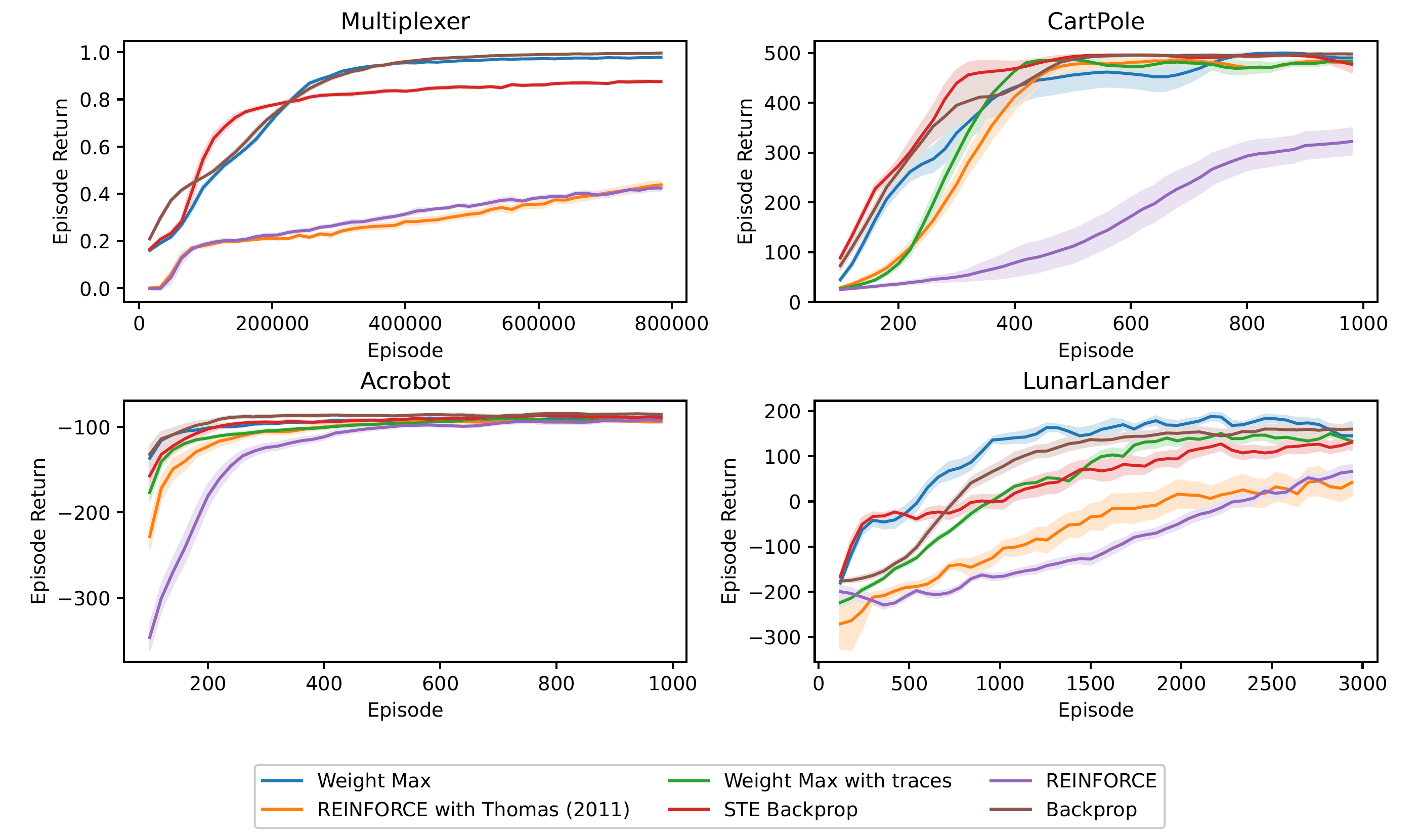
Our experiments show that the speed of Weight Maximization can roughly match the speed of STE backpropagation (straight-through backpropagation, which allows backpropagating through stochastic and discrete units) when applied to a network of Bernoulli logistic units in four standard RL tasks. We observe that Weight Maximization learns much faster than global REINFORCE, which indicates that Weight Maximization can effectively facilitate structural credit assignment. However, compared to a network of continuous-valued units trained by backpropagation, Weight Maximization performed slightly worse (except for the LunarLander task). This difference is likely due to the limitation of discrete-valued units - units can only communicate with binary values instead of real values.

Fig 3: Episode returns of networks of discrete units in different RL tasks. All networks are composed of Bernoulli logistic units except for backprop, where a network of continuous units is used. Results are averaged over 10 independent runs, and shaded areas represent standard deviation over the runs. Curves are smoothed with a running average of 100 episodes (10,000 episodes for the multiplexer task).

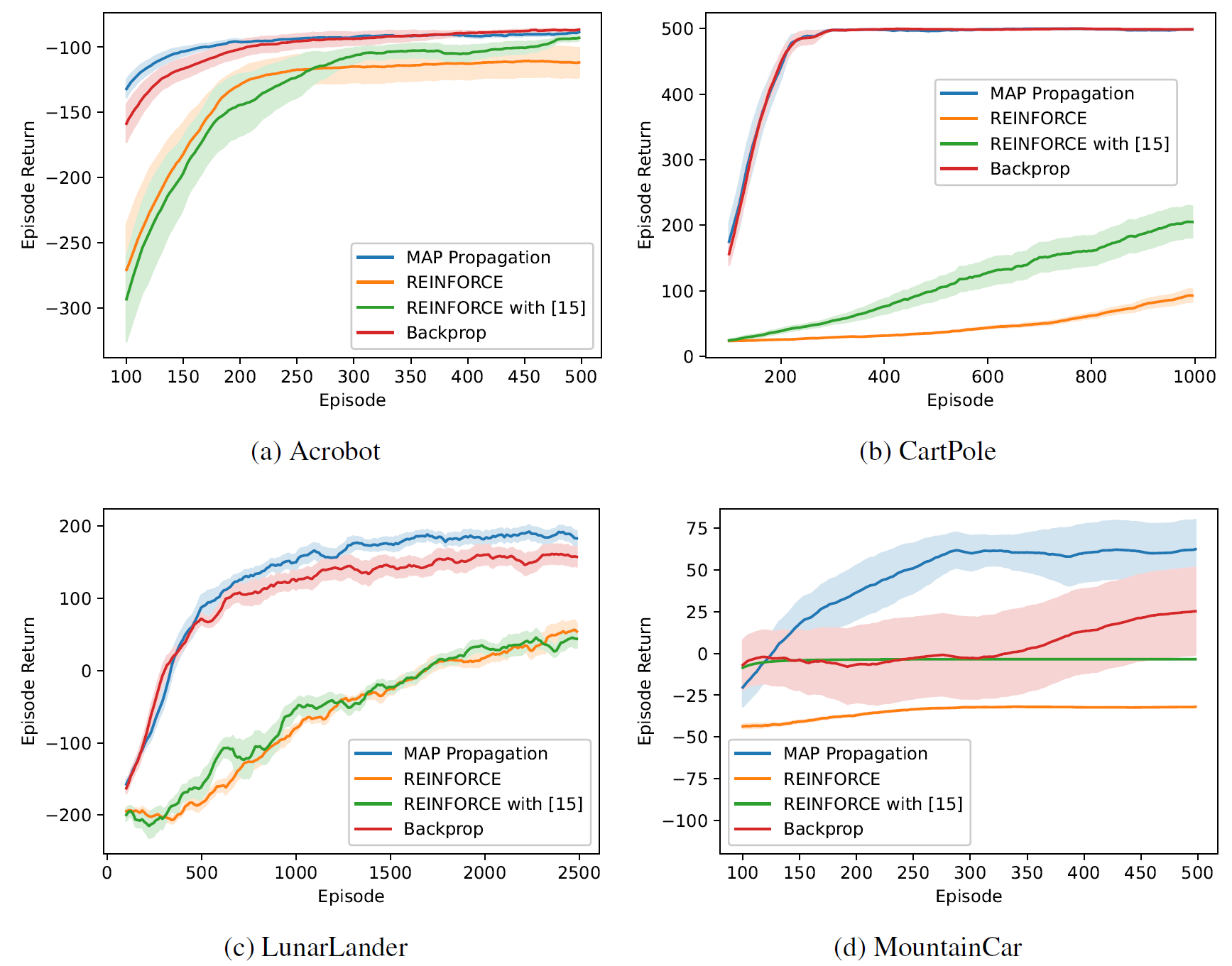
For networks of continuous-valued units, we also tested the performance of MAP Propagation and backpropagation on four standard RL tasks. Our experiment shows that MAP propagation can solve these tasks at a speed similar to that of backpropagation, and also agents trained by MAP propagation can avoid local optima better than backpropagation, as shown in the MountainCar task. This is the first work demonstrating that coagent networks can be trained at a speed similar to that of backpropagation.

Fig 4: Episode returns of networks of continuous units in different RL tasks. Results are averaged over 10 independent runs, and shaded areas represent standard deviation over the runs. Curves are smoothed with a running average of 100 episodes.

Conclusion

Besides their biological plausibility, coagent networks have distinct advantages. Firstly, coagent networks potentially enable better exploration. By introducing stochasticity at every level of the network, exploration can occur at higher levels than merely at the network’s outputs. This could equate to higher-level explorations, such as choosing to move a different chess piece, rather than just varying muscle twitches. Secondly, coagent networks may enhance robustness against perturbed inputs and help prevent overfitting. The inherent stochasticity at each network level necessitates greater adaptability, thereby forcing the network to become more resilient to variations in inputs.

This article introduces the concept of coagent networks and methods to facilitate structural credit assignment. We describe two learning methods, namely Weight Maximization and MAP Propagation, that can effectively speed up training in coagent networks so that their learning speed is similar to that of backpropagation. Both methods largely retain the biologically plausiblie property of Global REINFORCE. We hope that this research project may shed light on different methods of training neural networks and how biological neurons may perform structural credit assignments.

Ackowledgement

I am deeply grateful to have Andrew Barto as my supervisor, guiding me through this fascinating project.